
🍋 앙상블 알고리즘 - Boosting
1. Boosting
- 여러 트리 모델을 순차적으로 결합해서 오차를 줄이는 모델을 구성하는 방식
- 모델(tree)의 개수에 따라 예측 결과가 달라짐 (성능이 달라짐)
- 이전 모델이 잘못 예측한 데이터의 오차를 다음 모델에서 보완하도록 학습
- 병렬이 아닌 순차 학습 구조 → 학습 시간이 상대적으로 김
이전 모델이 틀린 부분에 더 집중해서 다음 모델을 학습하자!
2. Boosting - Gradient Boost
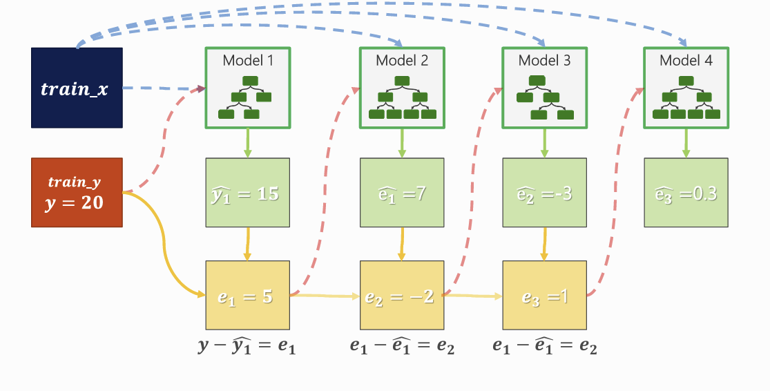
- 첫 번째 모델 : 단순 예측 수행
- 오차 계산 : 실제값 - 예측값
- 두 번째 모델 : 이전 모델의 오차를 예측하도록 학습
- 이 과정을 반복하면서 각 모델이 이전 모델의 부족한 부분을 보완
- 최종 예측값 : 모든 모델의 예측을 누적합으로 계산
3. Gradient Boost 수식 구하기
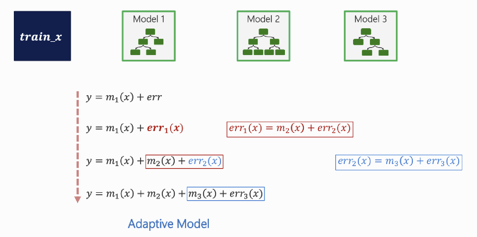
Fm(x)=Fm−1(x)+η⋅hm(x)
(𝜂 (learning rate) : 한 번에 얼마나 반영할지 조절하는 비율)
learning_rate 낮으면?
- 한 모델의 영향력 감소
- 더 많은 tree 필요
- 일반화 성능 증가
learning_rate 높으면?
- 빠른 학습
- 과적합 위험 증가
4. XGBoost
- Gradient Boosting을 속도 + 성능 + 안정성 측면에서 개선한 알고리즘
(1) XGBoost 특징
- 정규화(Regularization) 포함
- 결측값 자동 처리
- 분류 모델링 시, y는 정수 인코딩 필요: ['LEAVE', 'STAY'] -> [1, 0]
(2) 주요 파라미터
- learnign_rate: 조절 비율
- max_depth: tree의 depth 제한
- n_estimators: iteration 횟수
- subsample: 학습할 때, 샘플링 비율
- colsample_bytree: tree 만들 때 사용될 feature 비율
🍋 XGBoost 모델링 실습
1. 데이터 준비
(1) 라이브러리 불러오기
import pandas as pd
import numpy as np
import matplotlib.pyplot as plt
import seaborn as sns
from sklearn.model_selection import train_test_split
(2) 데이터 업로드
# mobile data
path = "https://@@@/mobile_cust_churn.csv"
data = pd.read_csv(path)
data.drop(['id', 'REPORTED_USAGE_LEVEL','OVER_15MINS_CALLS_PER_MONTH'], axis = 1, inplace = True)
data.rename(columns = {'HANDSET_PRICE':'H_PRICE',
                       'AVERAGE_CALL_DURATION':'DURATION',
                       'REPORTED_SATISFACTION':'SATISFACTION',
                       'CONSIDERING_CHANGE_OF_PLAN':'CHANGE'}
            , inplace = True)
data['CHURN'] = np.where(data['CHURN'] == 'LEAVE', 1, 0)  # XGBoost는 Label이 1,0 이어야 함
data.head()
# 데이터분할1
target = 'CHURN'
x = data.drop(target, axis=1)
y = data.loc[:, target]
# 가변수화
dumm_cols = ['SATISFACTION','CHANGE']
x = pd.get_dummies(x, columns = dumm_cols, drop_first = True)
# 데이터 분할2
x_train, x_val, y_train, y_val = train_test_split(x, y, test_size=.5, random_state = 20)2. 모델링
# 1) 함수 불러오기
from xgboost import XGBClassifier, plot_tree
from sklearn.metrics import *


# 2) 모델 선언 - 트리 개수 5개 & 깊이 3
model = XGBClassifier(n_estimators = 5, max_depth = 3)
# 3) 학습
model.fit(x_train, y_train)# 4) 예측
pred = model.predict(x_val)# 5) 평가
print(classification_report(y_val, pred)) precision recall f1-score support
0 0.68 0.74 0.71 5105
1 0.70 0.64 0.67 4895
accuracy 0.69 10000
macro avg 0.69 0.69 0.69 10000
weighted avg 0.69 0.69 0.69 100003. XGBoost
(1) 모델 시각화
xgboost에서 자체 plot_tree 함수를 제공함.
**plot_tree(model, num_tree=0)
plt.rcParams['figure.figsize'] = 20,20 # 그래프 크기 설정# 5개의 트리 중 4번째 트리 구조 시각화
plot_tree(model, num_trees = 4)
plt.show()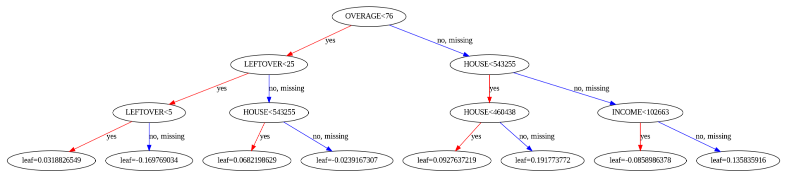
(2) 변수 중요도
# 변수 중요도
print(x_train.columns)
print(model.feature_importances_)
(3) 변수중요도 그래프 그리기 함수 만들기
def plot_feature_importance(importance, names):
    feature_importance = np.array(importance)
    feature_names = np.array(names)

    # 데이터프레임으로 정리
    data={'feature_names':feature_names,'feature_importance':feature_importance}
    fi_df = pd.DataFrame(data)

    # 중요도 기준 내림차순 정렬
    fi_df.sort_values(by=['feature_importance'], ascending=False,inplace=True)
    fi_df.reset_index(drop=True, inplace = True)

    plt.figure(figsize=(10,8))
    sns.barplot(x='feature_importance', y='feature_names', data = fi_df)

    plt.xlabel('FEATURE IMPORTANCE')
    plt.ylabel('FEATURE NAMES')
    plt.grid()


## 함수 실행
plot_feature_importance(model.feature_importances_, x_train.columns)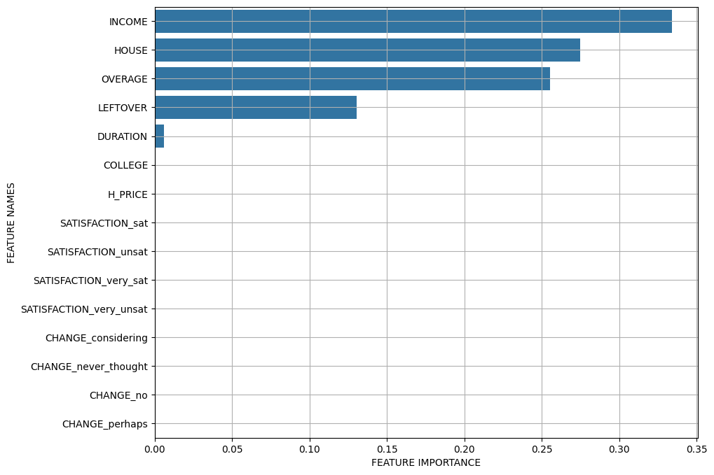
4. 하이퍼파라미터 변화에 따른 성능 추세
(1) n_estimators
from sklearn.model_selection import GridSearchCV

# 트리 개수를 1~99까지 테스트
grid_param = {'n_estimators':range(1,100,2)}

model = XGBClassifier()
model_gs = GridSearchCV(model, grid_param, cv = 5)

model_gs.fit(x_train, y_train)
# 교차검증 결과 저장
result = pd.DataFrame(model_gs.cv_results_)# 이 중에서 하이퍼파라미터 값에 따른 성능을 별도로 저장
temp = result.loc[:, ['param_n_estimators','mean_test_score']]
temp.head()# 성능 추이 시각화
plt.figure(figsize = (8,6))
sns.lineplot(x = 'param_n_estimators', y = 'mean_test_score', data = temp )
plt.grid()
plt.show()
# 어느순간까지는 성능이 올라가지만, 트리가 증가할수록 계속 떨어지는 경향을 보임
# 즉, 트리가 많다고 성능이 좋은게 아님 !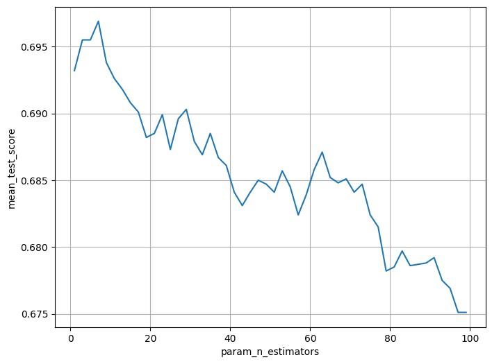
(2) learning rate
grid_param = {'learning_rate': np.linspace(0.02, 1, 50)}
model = XGBClassifier()
model_gs = GridSearchCV(model, grid_param, cv = 5)
model_gs.fit(x_train, y_train)
# 근데 위의 그래프에서 확인했을 때 7에서 가장 좋았으니까 그걸 넣어보자
grid_param = {'learning_rate': np.linspace(0.02, 1, 50)}
model_gs = GridSearchCV(model, grid_param, cv = 5)
model_gs.fit(x_train, y_train)result = pd.DataFrame(model_gs.cv_results_)temp = result.loc[:, ['param_learning_rate','mean_test_score']]
temp.head()plt.figure(figsize = (8,6))
sns.lineplot(x = 'param_learning_rate', y = 'mean_test_score', data = temp )
plt.grid()
plt.show()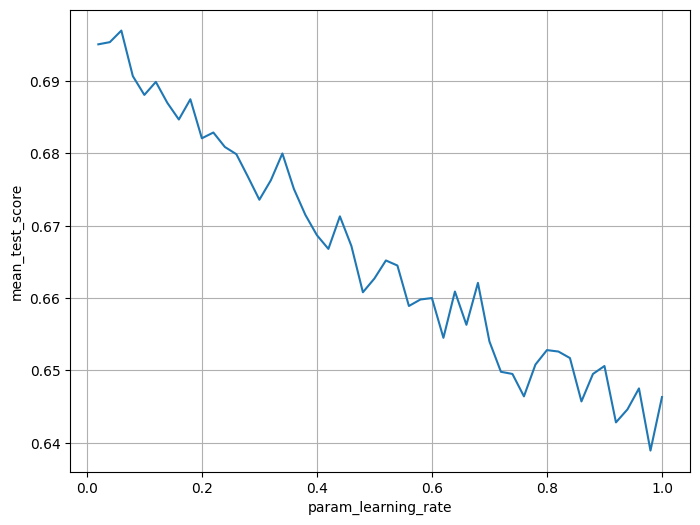
(3) n_estimators + learning rate 동시 튜닝
grid_param = {'learning_rate':np.linspace(0.01,0.3,30),
              'n_estimators':[3, 7, 15, 20, 30]}
model = XGBClassifier()
model_gs = GridSearchCV(model, grid_param, cv = 5)
model_gs.fit(x_train, y_train)
result = pd.DataFrame(model_gs.cv_results_)temp = result.loc[:, ['param_n_estimators', 'param_learning_rate','mean_test_score']]
temp.head()plt.figure(figsize = (8,6))
sns.lineplot(x = 'param_learning_rate', y = 'mean_test_score', data = temp, hue = 'param_n_estimators')
plt.grid()
plt.show()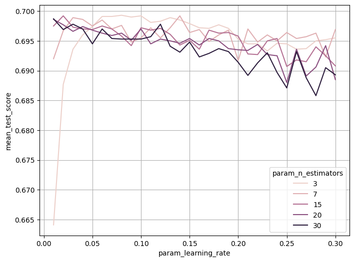
'BDA-11th' 카테고리의 다른 글
| [BDA 11기] 데이터 분석 모델링(ML1) - 14주차 (0) | 2026.02.02 |
|---|---|
| [BDA 11기] 데이터 분석 모델링(ML1) - 13주차 (0) | 2026.01.28 |
| [BDA 11기] 데이터 분석 모델링(ML1) - 11주차 (0) | 2026.01.15 |
| [BDA 11기] 데이터 분석 모델링(ML1) - 10주차 모델링 실습 (0) | 2026.01.06 |
| [BDA 11기] 데이터 분석 모델링(ML1) - 10주차 (0) | 2026.01.05 |